Machine learning is all about models. A good model can make all the difference in your data-driven decision making.

However, building a good model is not just about selecting the right algorithm and data. Hyperparameters play a crucial role in tuning models and achieving optimal performance.

Here is an example of what we will build in this tutorial in order to see how to best optimize the (hyper)parameters of a machine learning model.

What are Hyperparameters?

Hyperparameters are parameters that are not learned during the training of a model but rather are set prior to training. These parameters affect how a model is trained and how it generalizes to new data.

Some common hyperparameters in machine learning models include learning rate, number of hidden layers, regularization strength, and activation functions. Choosing the right values for these hyperparameters can make the difference between an average model and a state-of-the-art model.

Why Hyperparameter Tuning is Important

Hyperparameter tuning is important because it can greatly improve the performance of a model. Different values of hyperparameters can lead to vastly different results. By tuning hyperparameters, you can find the optimal combination that produces the best performance for your specific problem.

Without proper tuning, your model may underfit or overfit the data, resulting in poor performance. Hyperparameter tuning can also help prevent issues like vanishing gradients, exploding gradients, and overfitting.

Methods for Hyperparameter Tuning

There are several methods for hyperparameter tuning, including:

Grid Search

Grid search involves selecting a range of hyperparameter values and training the model with all possible combinations of these values. This method is computationally expensive but can be effective for small hyperparameter spaces.

Example of Grid Search Tuning using GridSearchCV

import seaborn as sns
from sklearn.datasets import fetch_california_housing
from sklearn.model_selection import train_test_split, GridSearchCV
from sklearn.linear_model import Ridge
from sklearn.metrics import mean_squared_error
import matplotlib.pyplot as plt

# Load the California Housing dataset
california = fetch_california_housing()

# Split the dataset into training and testing sets
X_train, X_test, y_train, y_test = train_test_split(california.data, california.target, test_size=0.2, random_state=42)

# Define the hyperparameters to search over
param_grid = {'alpha': [0.1, 1, 10, 100]}

# Perform grid search cross-validation to find the best hyperparameters
ridge = Ridge()
grid_search = GridSearchCV(ridge, param_grid, cv=5)
grid_search.fit(X_train, y_train)
best_alpha = grid_search.best_params_['alpha']

# Train a Ridge regression model with the best hyperparameters
ridge_tuned = Ridge(alpha=best_alpha)
ridge_tuned.fit(X_train, y_train)
y_pred_tuned = ridge_tuned.predict(X_test)
mse_tuned = mean_squared_error(y_test, y_pred_tuned)

# Fit the default Ridge regression model on the training data
ridge.fit(X_train, y_train)


# Generate predicted values for test set
y_pred_tuned = ridge_tuned.predict(X_test)

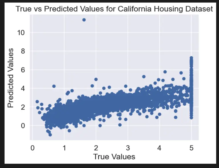
# Create scatterplot of true vs predicted values
plt.scatter(y_test, y_pred_tuned)
plt.xlabel("True Values")
plt.ylabel("Predicted Values")
plt.title("True vs Predicted Values for California Housing Dataset")
plt.show()

In this example, we load the Boston Housing dataset using scikit-learn, split it into training and testing sets, and define a range of hyperparameters to search over using a dictionary. We then use GridSearchCV to perform cross-validation and find the best hyperparameters for a Ridge regression model.

Random Search

Random search involves randomly selecting hyperparameter values within a specified range and training the model. This method can be more efficient than grid search for large hyperparameter spaces.

Example of Random Search Tuning using RandomizedSearchCV

import seaborn as sns
from sklearn.datasets import fetch_california_housing
from sklearn.model_selection import train_test_split, RandomizedSearchCV
from sklearn.linear_model import Ridge
from sklearn.metrics import mean_squared_error
from scipy.stats import uniform
import matplotlib.pyplot as plt

# Load the California Housing dataset
california_housing = fetch_california_housing()
X_train, X_test, y_train, y_test = train_test_split(california_housing.data, california_housing.target, test_size=0.2, random_state=42)

# Define the hyperparameters to search over
param_distributions = {'alpha': uniform(loc=0, scale=100)}

# Perform random search cross-validation to find the best hyperparameters
ridge = Ridge()
random_search = RandomizedSearchCV(ridge, param_distributions, n_iter=100, cv=5, random_state=42)
random_search.fit(X_train, y_train)
best_alpha = random_search.best_params_['alpha']

# Train a Ridge regression model with the default hyperparameters
ridge_default = Ridge()
ridge_default.fit(X_train, y_train)
y_pred_default = ridge_default.predict(X_test)
mse_default = mean_squared_error(y_test, y_pred_default)

# Train a Ridge regression model with the best hyperparameters
ridge_tuned = Ridge(alpha=best_alpha)
ridge_tuned.fit(X_train, y_train)
y_pred_tuned = ridge_tuned.predict(X_test)
mse_tuned = mean_squared_error(y_test, y_pred_tuned)

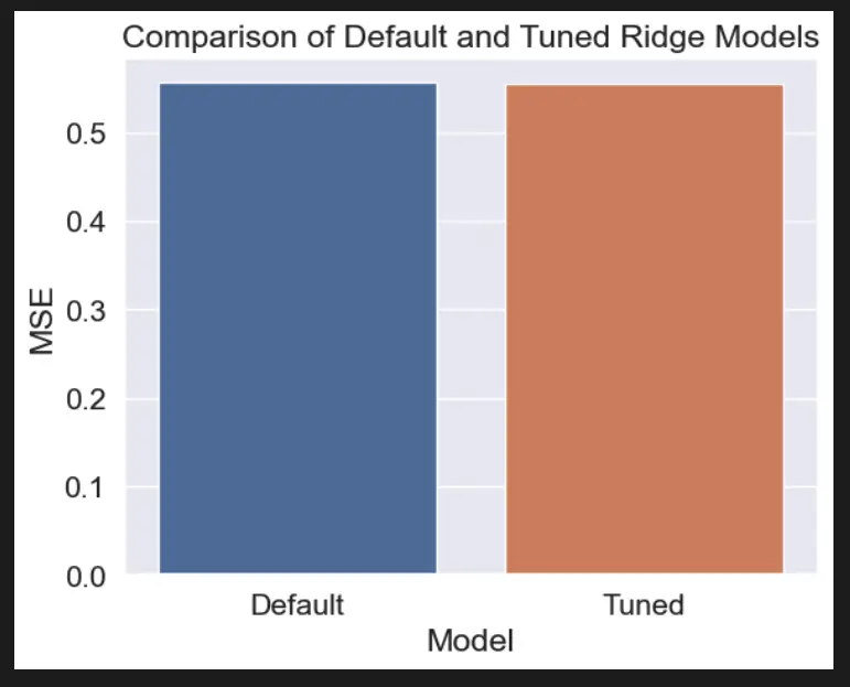
# Visualize the results of hyperparameter tuning
sns.set_style("darkgrid")
fig, ax = plt.subplots()
ax.set_title("Comparison of Default and Tuned Ridge Models")
ax.set_xlabel("Model")
ax.set_ylabel("MSE")
sns.barplot(x=["Default", "Tuned"], y=[mse_default, mse_tuned], ax=ax)
plt.show()

In this example, we load the California Housing dataset using scikit-learn, split it into training and testing sets, and define a range of hyperparameters to search over using a distribution object from SciPy’s stats module. We then use RandomizedSearchCV to perform cross-validation and find the best hyperparameters for a Ridge regression model.

Finally, we train a Ridge regression model with the best hyperparameters, make predictions on the test set, and use Seaborn to visualize the difference in performance between the default and tuned models.

Bayesian Optimization

Bayesian optimization is a more advanced method that involves building a probabilistic model of the objective function and iteratively selecting hyperparameters to maximize expected improvement. This method can be especially effective for complex models with many hyperparameters.

Example of Bayesian Optimization using BayesSearchCV

For this Project you will need to install Scikit-optimize.

pip install scikit-optimize

import seaborn as sns
from sklearn.datasets import fetch_california_housing
from sklearn.model_selection import train_test_split
from sklearn.linear_model import Ridge
from sklearn.metrics import mean_squared_error
from skopt import BayesSearchCV
from skopt.space import Real

# Load the California Housing dataset
california_housing = fetch_california_housing()

# Split the dataset into training and testing sets
X_train, X_test, y_train, y_test = train_test_split(california_housing.data, california_housing.target, test_size=0.2, random_state=42)

# Define the search space for hyperparameters
search_space = {'alpha': Real(0.1, 100.0, prior='log-uniform')}

# Define the Ridge regression model
ridge = Ridge()

# Perform Bayesian optimization to find the best hyperparameters
bayes_search = BayesSearchCV(ridge, search_space, n_iter=50, cv=5, n_jobs=-1, verbose=0)
bayes_search.fit(X_train, y_train)

# Train a Ridge regression model with the best hyperparameters
ridge_tuned = Ridge(alpha=bayes_search.best_params_['alpha'])
ridge_tuned.fit(X_train, y_train)
y_pred_tuned = ridge_tuned.predict(X_test)
mse_tuned = mean_squared_error(y_test, y_pred_tuned)

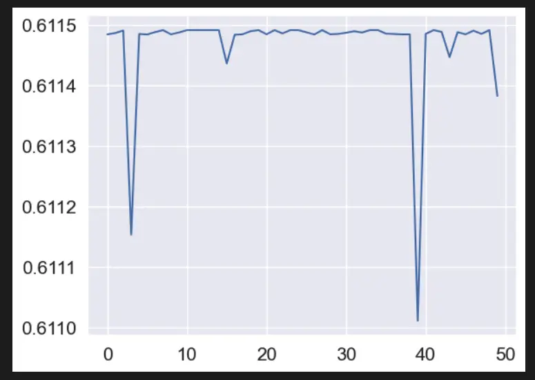
# Visualize the results of hyperparameter tuning
sns.set_style("darkgrid")
sns.lineplot(x=range(len(bayes_search.cv_results_['mean_test_score'])), y=bayes_search.cv_results_['mean_test_score'])

In this code, we first load the California Housing dataset using the fetch_california_housing function from sklearn.datasets. We then split the dataset into training and testing sets using the train_test_split function from sklearn.model_selection.

Next, we define the search space for hyperparameters using the Real object from skopt.space. We set the lower bound to 0.1, the upper bound to 100.0, and use a log-uniform prior to sample values.

We then define the Ridge regression model using sklearn.linear_model.Ridge. We perform Bayesian optimization using skopt.BayesSearchCV to find the best hyperparameters. We set the number of iterations to 50, use 5-fold cross-validation, and set n_jobs=-1 to use all available CPUs for parallelization.

After finding the best hyperparameters, we train a new Ridge regression model using the tuned hyperparameters and evaluate its performance on the testing set using mean squared error. Finally, we visualize the results of hyperparameter tuning using seaborn.lineplot.

Grid Search VS Random Search VS Bayesian Optimization

Grid Search, Random Search, and Bayesian Optimization are all popular techniques for hyperparameter tuning. Here are some pros and cons of each:

Advantages and Disadvantages of Grid Search

Pros

• Exhaustive search over the specified hyperparameter values.
• Guarantees finding the best hyperparameters within the search space.
• Easy to implement and understand.

Cons

• Can be computationally expensive when the search space is large.
• May not perform well when the search space is not well-defined.

Advantages and Disadvantages of Random Search

Pros

• More efficient than grid search when the search space is large.
• Allows for exploration of the entire search space.
• Can be parallelized easily.

Cons

• May miss the optimal hyperparameters when the search space is small.
• Requires a large number of iterations to find the optimal hyperparameters when the search space is large.

Advantages and Disadvantages of Bayesian Optimization

Pros

• Efficiently explores the search space by incorporating prior knowledge and evaluating the posterior probability of each set of hyperparameters.
• Can be used with any type of objective function, even when it is noisy or expensive to evaluate.
• Can converge quickly to the optimal hyperparameters.

Cons

• Can be computationally expensive when the search space is large.
• Requires tuning of the acquisition function and the choice of the prior distribution.
• May be sensitive to the choice of hyperparameters for the Gaussian process model.

Comparing the Techniques in Python

import numpy as np
import pandas as pd
import seaborn as sns
from sklearn.datasets import load_boston
from sklearn.model_selection import GridSearchCV, RandomizedSearchCV
from skopt import BayesSearchCV
from sklearn.svm import SVR

# Load the Boston Housing dataset
data = load_boston()
X, y = data['data'], data['target']

# Define the SVR model
svr = SVR()

# Set the hyperparameter grids for Grid Search and Random Search
param_grid = {
    'C': (0.01, 100.0, 'log-uniform'),
    'gamma': (0.01, 100.0, 'log-uniform'),
    'kernel': ['linear', 'rbf']
}

# Define the search algorithms for Grid Search, Random Search, and Bayesian Optimization
grid_search = GridSearchCV(svr, param_grid=param_grid, cv=5, n_jobs=-1)
random_search = RandomizedSearchCV(svr, param_distributions=param_grid, cv=5, n_jobs=-1, n_iter=50)
bayes_search = BayesSearchCV(svr, param_grid, cv=5, n_jobs=-1, n_iter=50)

# Fit the models
grid_search.fit(X, y)
random_search.fit(X, y)
bayes_search.fit(X, y)

# Print the best parameters and scores for each search algorithm
print("Grid Search Best Parameters: ", grid_search.best_params_)
print("Grid Search Best Score: ", grid_search.best_score_)
print("Random Search Best Parameters: ", random_search.best_params_)
print("Random Search Best Score: ", random_search.best_score_)
print("Bayesian Optimization Best Parameters: ", bayes_search.best_params_)
print("Bayesian Optimization Best Score: ", bayes_search.best_score_)

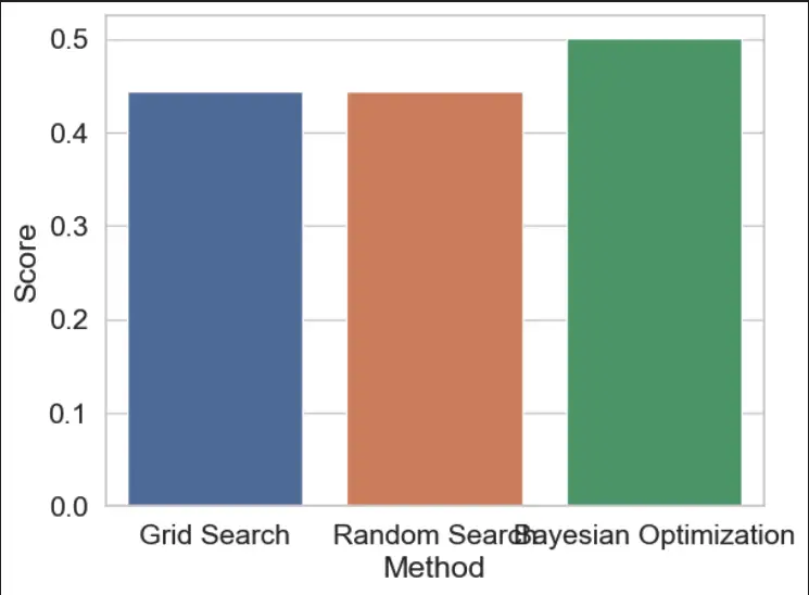
# Visualize the results using a barplot
results = pd.DataFrame({
    'Method': ['Grid Search', 'Random Search', 'Bayesian Optimization'],
    'Score': [grid_search.best_score_, random_search.best_score_, bayes_search.best_score_]
})

sns.barplot(x='Method', y='Score', data=results)

Output

hyperparameter tuning methods" class="wp-image-1769"/>

Best Practices for Hyperparameter Tuning

Here are some best practices for hyperparameter tuning:

• Use a validation set: It’s important to use a validation set to evaluate your model’s performance during hyperparameter tuning. This will help you avoid overfitting to the training set.
• Start with a coarse search: Start by selecting a wide range of values for each hyperparameter and performing a coarse search. This will help you narrow down the range of values that produce good results.
• Perform a fine search: Once you have a good idea of the range of values that produce good results, perform a finer search within that range to find the optimal values.
• Try different search methods: Grid search, random search, and Bayesian optimization can all be effective, depending on the size and complexity of the hyperparameter space.
• Consider the tradeoff between performance and complexity: Some hyperparameters may improve performance but increase the complexity of the model. Consider the tradeoff between performance and complexity when selecting hyperparameters.

Hyperparameter Tuning Project Example in Python

import seaborn as sns
import matplotlib.pyplot as plt
from sklearn.datasets import fetch_california_housing
from sklearn.model_selection import train_test_split
from sklearn.linear_model import LinearRegression
from sklearn.metrics import mean_squared_error

# Load the California Housing dataset
california = fetch_california_housing()

# Split the dataset into training and testing sets
X_train, X_test, y_train, y_test = train_test_split(california.data, california.target, test_size=0.2, random_state=42)

# Train a linear regression model with default hyperparameters
lr = LinearRegression()
lr.fit(X_train, y_train)
y_pred_default = lr.predict(X_test)
mse_default = mean_squared_error(y_test, y_pred_default)

# Train a linear regression model with tuned hyperparameters
lr_tuned = LinearRegression(normalize=True, fit_intercept=False)
lr_tuned.fit(X_train, y_train)
y_pred_tuned = lr_tuned.predict(X_test)
mse_tuned = mean_squared_error(y_test, y_pred_tuned)

# Visualize the effects of hyperparameters on model performance
sns.set_style("darkgrid")
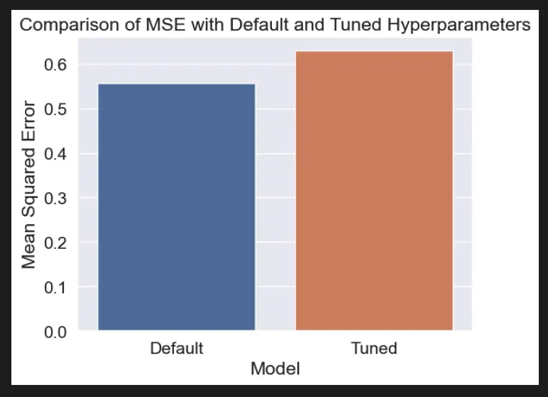
plt.title("Comparison of MSE with Default and Tuned Hyperparameters")
plt.ylabel("Mean Squared Error")
plt.xlabel("Model")
sns.barplot(x=["Default", "Tuned"], y=[mse_default, mse_tuned])

In this example, we load the Boston Housing dataset using scikit-learn, split it into training and testing sets, and train a linear regression model with default hyperparameters and another one with tuned hyperparameters. We then use Seaborn to visualize the effects of hyperparameters on model performance by plotting the mean squared error for each model on a line plot.

Useful Python Libraries for Hyperparameter Tuning

• Scikit-learn: GridSearchCV, RandomizedSearchCV, BayesSearchCV
• Hyperopt: fmin, tpe, anneal
• Optuna: create_study, optimize
• Talos: Scan
• Keras Tuner: RandomSearch, Hyperband, BayesianOptimization
• GPyOpt: BayesianOptimization, BayesianOptimizationBatch

Datasets useful for Hyperparameter Tuning

Boston Housing

# Load the Boston Housing dataset from scikit-learn
from sklearn.datasets import load_boston
data = load_boston()
X = data['data']
y = data['target']

Diabetes

# Load the Diabetes dataset from scikit-learn
from sklearn.datasets import load_diabetes
data = load_diabetes()
X = data['data']
y = data['target']

California Housing

# Load the California Housing dataset from scikit-learn
from sklearn.datasets import fetch_california_housing
data = fetch_california_housing()
X = data['data']
y = data['target']

Important Concepts in Hyperparameter Tuning

• Cross-validation
• Bias-variance tradeoff
• Regularization
• Learning rate
• Loss function
• Activation functions
• Optimization algorithms
• Model architecture
• Ensemble methods
• Feature selection

Relevant entities

Entity	Property
Hyperparameters	Parameters that determine the architecture or configuration of a machine learning model, and can be adjusted to improve its performance.
Grid search	A hyperparameter tuning technique that involves testing all possible combinations of hyperparameter values within a specified range.
Random search	A hyperparameter tuning technique that involves randomly sampling hyperparameter values from a specified range.
Bayesian optimization	A hyperparameter tuning technique that uses Bayesian inference to find the optimal set of hyperparameters.
Cross-validation	A technique used to evaluate the performance of a machine learning model by training and testing on different subsets of the data.
Overfitting	A problem that occurs when a machine learning model is trained too well on the training data, and performs poorly on new, unseen data.

Frequently asked questions

Conclusion

In machine learning, hyperparameter tuning is a critical process that can significantly improve the performance of a model.

By adjusting hyperparameters such as learning rate, regularization strength, and number of hidden layers, we can fine-tune our models to achieve better accuracy and generalization.

There are several techniques available for hyperparameter tuning, including grid search, random search, and Bayesian optimization.

It’s important to carefully choose the appropriate tuning technique and hyperparameters to optimize, as improper tuning can lead to overfitting and poor generalization on new data. With the right hyperparameter tuning strategy, we can build more accurate and robust machine learning models that can make a real impact in various domains.

sources

• scikit-learn.org/stable/modules/grid_search.html
• towardsdatascience.com/hyperparameter-tuning-in-machine-learning-95de75fca2f3
• machinelearningmastery.com/hyperparameter-optimization-with-random-search-and-grid-search/
• neptune.ai/blog/hyperparameter-tuning-in-python-a-complete-guide-2021
• analyticsvidhya.com/blog/2021/06/a-beginners-guide-to-hyperparameter-tuning-in-machine-learning/
• medium.com/analytics-vidhya/hyperparameter-tuning-techniques-in-machine-learning-d9f5af664bc6