
In machine learning, building a model is a crucial step to make predictions based on the given data. However, it is important to be mindful of the two types of errors that may occur: overfitting and underfitting. Overfitting happens when the model becomes too complex that it fits perfectly on the training data, but performs poorly on the new, unseen data. Meanwhile, underfitting occurs when the model is too simple to capture the patterns in the data, resulting in poor performance on both training and testing data.
In this article, we will explore the concepts of overfitting and underfitting in machine learning, their causes, and how to address them.
What is Overfitting?
Overfitting happens when the model captures the noise in the training data and fits too closely to it, resulting in a model that performs well on the training data but poorly on the new data. The model essentially memorizes the training data, making it unable to generalize to new data.
Causes of Overfitting
One common cause of overfitting is using a model that is too complex for the amount of available data. For example, fitting a polynomial of degree 20 with only 10 data points would likely result in overfitting.
Another cause of overfitting is when there is noise in the training data. In this case, the model might fit the noise instead of the underlying pattern, leading to poor performance on new data.
How to Address Overfitting
One common technique to address overfitting is regularization, which involves adding a penalty term to the loss function. This penalty term discourages the model from fitting the noise in the data and encourages it to generalize better to new data.
Another approach is to use early stopping during the training process. Early stopping involves stopping the training when the performance on the validation data starts to decrease. This technique prevents the model from continuing to fit the training data too closely.
What is Underfitting?
Underfitting occurs when the model is too simple and unable to capture the underlying patterns in the data, resulting in poor performance on both the training and new data.
Causes of Underfitting
Underfitting may occur when using a model that is too simple or has too few parameters. For example, fitting a linear model to data that has a complex, nonlinear relationship would likely result in underfitting.
Another cause of underfitting is when the training data is insufficient to capture the underlying patterns in the data.
How to Address Underfitting
One common approach to address underfitting is to use a more complex model. This may involve increasing the number of parameters in the model or using a more sophisticated model architecture.
Another approach is to increase the amount of training data available to the model. This may help the model to better capture the underlying patterns in the data.
Conclusion
Overfitting and underfitting are common problems in machine learning, and addressing them is crucial to building models that can generalize well to new data. Regularization and early stopping can help prevent overfitting, while using a more complex model or increasing the amount of data can help address underfitting. It is important to strike a balance between the complexity of the model and the amount of available data to avoid these issues and build a model that performs well on new data.
Useful Python Libraries for Overfitting and underfitting
- Scikit-learn: train_test_split, KFold, GridSearchCV
- TensorFlow: Dropout, EarlyStopping
- PyTorch: Dropout, EarlyStopping
- Matplotlib: plot, scatter, subplot, legend
Datasets useful for Overfitting and underfitting
California Housing Dataset
from sklearn.datasets import fetch_california_housing
#Load California Housing dataset
california_housing = fetch_california_housing()

#Split the dataset into train and test sets
from sklearn.model_selection import train_test_split
X_train, X_test, y_train, y_test = train_test_split(california_housing.data, california_housing.target, test_size=0.2, random_state=42)
Python Example
from sklearn.preprocessing import PolynomialFeatures
from sklearn.linear_model import LinearRegression
import numpy as np
import matplotlib.pyplot as plt
# Generate some synthetic data
np.random.seed(0)
n_samples = 30
X = np.sort(np.random.rand(n_samples))
y = np.sin(2 * np.pi * X) + np.random.randn(n_samples) * 0.1
# Define the degrees of the polynomial to fit
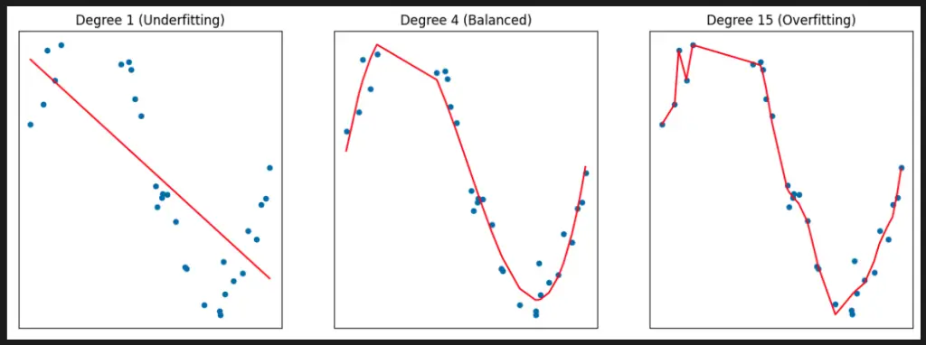
degrees = [1, 4, 15]
# Fit and plot the polynomial regression models
plt.figure(figsize=(15, 5))
for i, degree in enumerate(degrees):
ax = plt.subplot(1, len(degrees), i + 1)
plt.setp(ax, xticks=(), yticks=())
# Transform the input features to include polynomial terms up to degree
poly = PolynomialFeatures(degree=degree, include_bias=False)
X_poly = poly.fit_transform(X.reshape(-1, 1))
# Fit a linear regression model to the polynomial features
model = LinearRegression()
model.fit(X_poly, y)
# Plot the data and the polynomial regression curve
plt.scatter(X, y, s=20)
plt.plot(X, model.predict(X_poly), color='r')
if degree == 1:
plt.title(f'Degree {degree} (Underfitting)')
elif degree == 4:
plt.title(f'Degree {degree} (Balanced)')
elif degree == 15:
plt.title(f'Degree {degree} (Overfitting)')
plt.show()
This code generates some synthetic data and fits polynomial regression models of different degrees to the data, plotting the results to visualize the effect of overfitting and underfitting. The PolynomialFeatures class is used to transform the input features to include polynomial terms up to a specified degree, and the LinearRegression class is used to fit a linear regression model to the transformed features. The resulting curves show how increasing the degree of the polynomial can lead to overfitting, where the model becomes too complex and fits the noise in the data, or underfitting, where the model is too simple and fails to capture the underlying pattern in the data.

This code fits a 12-degree polynomial regression model to the Boston Housing dataset and plots the predicted values against the true values for both the training and testing sets. The plot also includes lines for the ideal model and the training and testing errors.
To Know Before You Learn Overfitting and underfitting?
- Understanding of basic machine learning concepts and algorithms.
- Familiarity with Python programming language and relevant libraries such as Scikit-learn and Matplotlib.
- Knowledge of data pre-processing and feature engineering techniques.
- Understanding of model evaluation metrics such as accuracy, precision, recall, and F1 score.
- Familiarity with the bias-variance trade-off concept.
Important Concepts in Overfitting and underfitting
- Bias-Variance Tradeoff
- Regularization
- Cross-Validation
- Model Complexity
- Training Set vs. Test Set
- Learning Curves
Relevant entities
| Entities | Properties |
|---|---|
| Model Complexity | High complexity models overfit, while low complexity models underfit |
| Training Data | The dataset used to train the model |
| Validation Data | The dataset used to tune the model’s hyperparameters |
| Generalization Error | The error rate on unseen data |
| Bias | Error due to the model’s inability to represent the true function |
| Variance | Error due to the model’s sensitivity to the training data |
Sources:
- https://en.wikipedia.org/wiki/Overfitting
- https://en.wikipedia.org/wiki/Underfitting
- https://www.analyticsvidhya.com/blog/2020/02/what-is-overfitting-in-machine-learning/
- https://machinelearningmastery.com/overfitting-and-underfitting-with-machine-learning-algorithms/
- https://towardsdatascience.com/understanding-overfitting-and-underfitting-in-deep-learning-896baddd4d5c
