Principal Component Analysis (PCA) is a dimensionality reduction technique that is widely used in machine learning, computer vision, and data analysis.

It is a mathematical method that transforms high-dimensional data into a low-dimensional representation while retaining as much of the original information as possible.

PCA finds the most important features of the data, called principal components, and expresses the data in terms of those components.

Relevant Definitions

Entity	Properties
PCA	Principal Component Analysis is a dimensionality reduction technique that finds the most important features of a dataset and expresses the data in terms of those features.
Covariance matrix	A square matrix that shows how each variable in the data is related to every other variable.
Eigenvectors	Directions in which the data varies the most. These are used to create a new coordinate system for the data.
Eigenvalues	Indicate how much variance there is in the data along each eigenvector.
Dimensionality reduction	The process of reducing the number of variables in a dataset, while retaining as much information as possible.
Data visualization	The process of representing high-dimensional data in a lower-dimensional space, while preserving as much information as possible.
Feature extraction	The process of extracting the most important features of a dataset, which can be used as input to a machine learning algorithm.
Noise reduction	The process of removing noise from a dataset, which can improve the performance of machine learning algorithms.
Preprocessing	The process of transforming the data to prepare it for analysis, such as by removing outliers or scaling the data.

Why learn Principal Component Analysis (PCA)?

Learning about Principal Component Analysis (PCA) can be valuable for a number of reasons:

1. Dimensionality Reduction: PCA is a powerful tool for reducing the number of variables in a dataset, while retaining as much information as possible. This can be particularly useful in machine learning, where high-dimensional data can be difficult to work with.
2. Data Visualization: PCA can be used to visualize high-dimensional data in a lower-dimensional space. This can be particularly useful for gaining insights into the structure of the data.
3. Feature Extraction: PCA can be used to extract the most important features of a dataset, which can be used as input to a machine learning algorithm.
4. Noise Reduction: PCA can be used to remove noise from a dataset, which can improve the performance of machine learning algorithms.
5. Preprocessing: PCA can be used as a preprocessing step for machine learning algorithms, which can improve their performance by reducing the number of variables and removing noise.

Overall, learning about PCA can be valuable for anyone working with high-dimensional data, particularly in the fields of machine learning, computer vision, and data analysis.

Applications of PCA

PCA has a wide range of applications, including:

• Image compression and feature extraction in computer vision
• Noise reduction in signal processing
• Data visualization in data analysis
• Dimensionality reduction in machine learning

How does PCA Work (Python Explained)?

The goal of PCA is to transform a dataset with many variables into a dataset with fewer variables, while preserving as much of the original information as possible.

PCA does this by finding a new set of variables that are linear combinations of the original variables, and are uncorrelated with each other. These new variables are called principal components.

PCA finds the principal components by first calculating the covariance matrix of the data.

import numpy as np

# Create a matrix
A = np.array([[1, 2], [2, 3], [3, 4]])
print('Data:\n',A)

# Calculate the covariance matrix
cov_mat = np.cov(A.T)
print('Covariance Matrix:\n',cov_mat)

The covariance matrix shows how each variable in the data is related to every other variable. PCA then finds the eigenvectors and eigenvalues of this covariance matrix (square matrix giving the covariance between each pair of elements).

The eigenvectors and eigenvalues are used to create a new coordinate system for the data.

The eigenvectors are the directions in which the data varies the most, and the eigenvalues indicate how much variance there is in the data along each eigenvector.

# Sort eigenvalues in decreasing order
idx = eigenvalues.argsort()[::-1]
eigenvalues = eigenvalues[idx]
eigenvectors = eigenvectors[:, idx]
print('Eigenvalues:\n', eigenvalues)
print('Eigenvectors:\n', eigenvectors)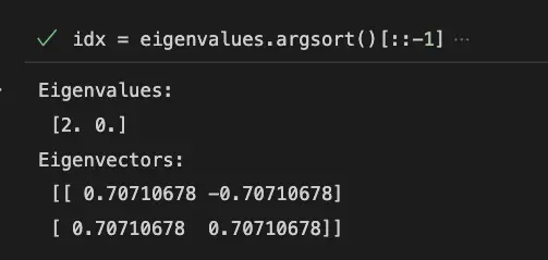

The first principal component is the direction in which the data varies the most, and each subsequent principal component is orthogonal to the previous ones and captures the next most variance in the data.

The data is then projected onto this new coordinate system, which results in a new dataset with fewer variables.

# Transform the data using the eigenvectors
transformed = A.dot(eigenvectors)

# Print the transformed data
print('Transformed:\n', transformed)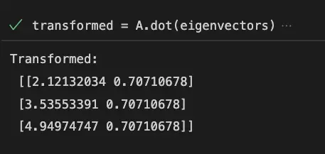   

Limitations of PCA

Although PCA is a powerful technique, it has some limitations:

• PCA assumes that the data is linearly related, which may not always be the case
• PCA may not work well if the variables in the data are not normally distributed
• PCA may not work well if the data contains outliers
• PCA may not always be able to capture the most important features of the data, especially if the data is highly non-linear

Python code Examples

scikit-learn">PCA Implementation using scikit-learn

from sklearn.decomposition import PCA
from sklearn.datasets import load_iris
#Load iris dataset
iris = load_iris()

#Create PCA object
pca = PCA(n_components=2)

#Fit the data
iris_pca = pca.fit_transform(iris.data)

#Print the explained variance ratio
print(pca.explained_variance_ratio_)

Here is the output:

This example shows how to perform PCA using scikit-learn library in Python. The iris dataset is loaded and a PCA object is created with 2 principal components. The data is then fitted to the PCA object and transformed to the new coordinate system. The explained variance ratio is printed to show the amount of variance retained by each principal component. For more information and examples, you can visit scikit-learn documentation.

scikit-learn">Scree plot with PCA using scikit-learn

import numpy as np
import matplotlib.pyplot as plt
from sklearn.datasets import load_digits
from sklearn.decomposition import PCA

# Load data
digits = load_digits()

# Initialize PCA with 2 components
pca = PCA(n_components=2)

# Fit and transform data
X_pca = pca.fit_transform(digits.data)

# Compute explained variance ratio
explained_variance_ratio = pca.explained_variance_ratio_

# Compute cumulative explained variance ratio
cumulative_explained_variance_ratio = np.cumsum(explained_variance_ratio)

# Plot scree plot
plt.bar(
    range(1, len(explained_variance_ratio) + 1), 
    explained_variance_ratio, 
    label='Explained Variance Ratio'
        )
plt.plot(range(1, len(cumulative_explained_variance_ratio) + 1), cumulative_explained_variance_ratio, 'ro-', label='Cumulative Explained Variance Ratio')
plt.xlabel('Principal Component')
plt.ylabel('Explained Variance Ratio')
plt.title('Scree Plot with PCA')
plt.legend()
plt.show()

Output:

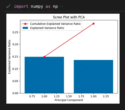
This code shows how to create a scree plot with PCA using scikit-learn. The scree plot is a graph that shows the amount of variance explained by each principal component. The x-axis shows the number of principal components, while the y-axis shows the percentage of variance explained. The scree plot is useful for determining the optimal number of principal components to retain.

PCA Scatterplot on the Digits Dataset

import seaborn as sns
from sklearn.datasets import load_digits
from sklearn.decomposition import PCA

digits = load_digits()

# Perform PCA
pca = PCA(n_components=2)
projected = pca.fit_transform(digits.data)

# Create scatterplot with seaborn
sns.scatterplot(x=projected[:, 0], y=projected[:, 1], hue=digits.target, legend="full", palette="viridis")

Output:

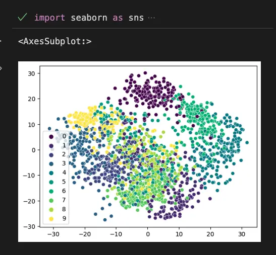
This code uses the seaborn library to create a scatterplot of the 2 principal components obtained from the digits dataset using PCA. The load_digits() function is used to load the dataset, and PCA is used to perform the PCA with 2 components. Finally, the sns.scatterplot() function is used to create the scatterplot with the principal components on the x and y axes, the target variable as the color, and a viridis color palette.

Reduce Noise on the Digits Dataset

import numpy as np
import matplotlib.pyplot as plt
from sklearn.datasets import load_digits
from sklearn.decomposition import PCA

# Load the digits dataset
digits = load_digits()

# Add noise to the dataset
np.random.seed(0)
noisy_digits = digits.data + np.random.normal(0, 4, size=digits.data.shape)

# Fit PCA to the noisy dataset
pca = PCA(0.01) # Retain 1% of the variance
components = pca.fit_transform(noisy_digits)
filtered_digits = pca.inverse_transform(components)

# Plot the noisy and filtered digits
fig, ax = plt.subplots(2, 10, figsize=(10, 2))
for i in range(10):
    ax[0, i].imshow(noisy_digits[i].reshape(8, 8), cmap='gray')
    ax[1, i].imshow(filtered_digits[i].reshape(8, 8), cmap='gray')
    ax[0, i].axis('off')
    ax[1, i].axis('off')
ax[0, 0].set_title('Noisy')
ax[1, 0].set_title('Filtered')
plt.show()

Output:

Eigenvalues and Eigenvectors

In PCA, eigenvalues and eigenvectors are used to transform the original features into new uncorrelated variables called principal components.

• Eigenvalues represent the magnitude of the variance of each principal component.
• Eigenvectors represent the direction or pattern of the data in each principal component.

Here’s a Python example of how to calculate eigenvalues and eigenvectors using NumPy:

Python Example

import numpy as np

# Create a matrix
A = np.array([[1, 2, 3], [4, 5, 6], [7, 8, 9]])

# Calculate the eigenvalues and eigenvectors of A
eigenvalues, eigenvectors = np.linalg.eig(A)

# Print the eigenvalues and eigenvectors
print("Eigenvalues:\n", eigenvalues)
print("\nEigenvectors:\n", eigenvectors)

Output:

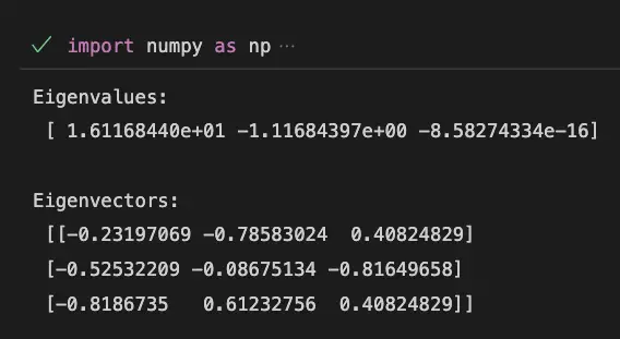
In this example, the eigenvalues represent the variance of the three principal components, and the eigenvectors represent the direction or pattern of the data in each principal component.

Covariance Matrix in PCA

In PCA, the covariance matrix is used to identify the directions in which the data varies the most. It is a square matrix that contains the variances and covariances of the different features in the data. The diagonal elements of the covariance matrix represent the variance of each feature, while the off-diagonal elements represent the covariance between different pairs of features.

To compute the covariance matrix in Python using the digits dataset, we can use the numpy library as follows:

import numpy as np
from sklearn.datasets import load_digits

# Load the digits dataset
digits = load_digits()

# Compute the covariance matrix
X = digits.data
X_mean = np.mean(X, axis=0)
X_centered = X - X_mean
cov_matrix = np.cov(X_centered.T)  
cov_matrix

In the code above, we first load the digits dataset using load_digits() from the sklearn.datasets module. We then compute the covariance matrix by first subtracting the mean of each feature from the data (X_centered), and then using np.cov() to compute the covariance matrix (cov_matrix) of the centered data. We transpose the centered data (X_centered.T) because np.cov() expects each row to represent an observation and each column to represent a feature.

The resulting cov_matrix will be a 64×64 matrix, since the digits dataset has 64 features.

Singular value decomposition (SVD) in PCA

Singular Value Decomposition (SVD) is a matrix factorization method that is often used in PCA to reduce the dimensionality of a dataset. It decomposes a matrix into three parts: the left singular vectors, the right singular vectors, and the singular values.

In PCA, the SVD is applied to the covariance matrix of the data to obtain the principal components. The left singular vectors correspond to the principal components, while the singular values represent the amount of variance captured by each principal component.

Here’s an example of how to perform SVD on the digits dataset in Python using the NumPy library:

import numpy as np
from sklearn.datasets import load_digits

# Load the digits dataset
digits = load_digits()

# Get the data
X = digits.data

# Calculate the covariance matrix
covariance_matrix = np.cov(X.T)

# Perform SVD on the covariance matrix
U, s, Vt = np.linalg.svd(covariance_matrix)

# Get the principal components
components = U

# Get the explained variance
explained_variance = s ** 2 / (len(X) - 1)

# Get the total explained variance
total_explained_variance = np.sum(explained_variance)

# Print the results
print("Principal components:\n", components)
print("Explained variance:\n", explained_variance)
print("Total explained variance:", total_explained_variance)

Output:

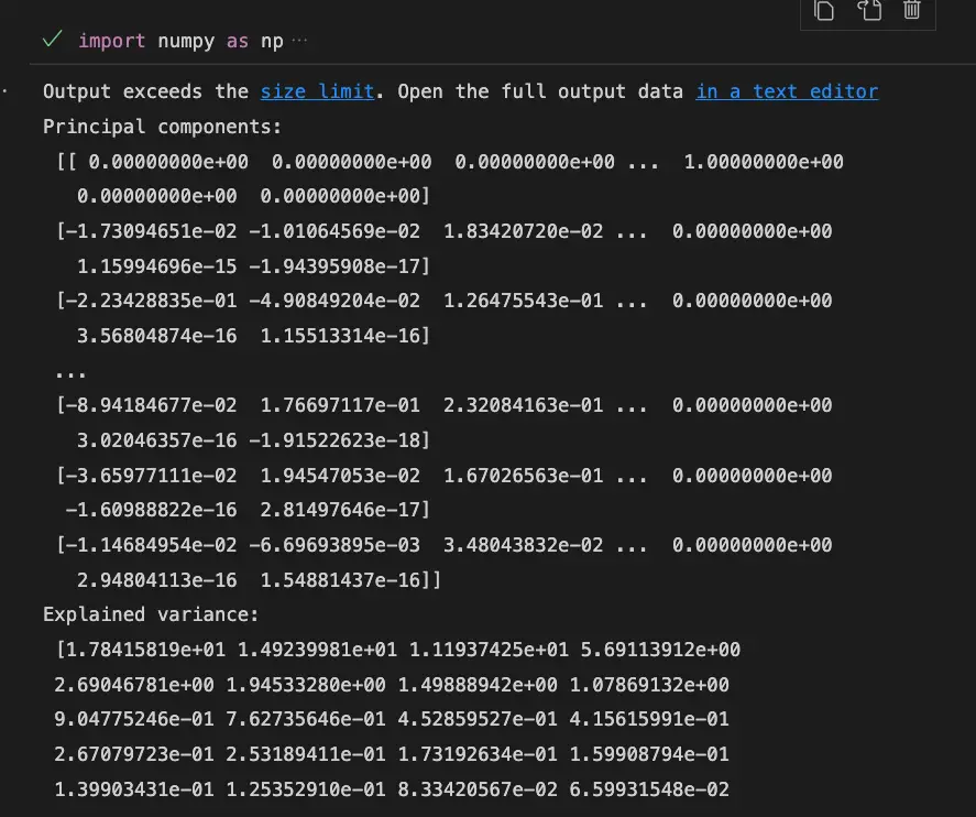
In this example, we first load the digits dataset using the load_digits function from the sklearn.datasets module. Then, we get the data and calculate the covariance matrix using the np.cov function from the NumPy library.

Next, we perform SVD on the covariance matrix using the np.linalg.svd function from NumPy. This returns the left singular vectors in U, the singular values in s, and the right singular vectors in the transpose of V.

We then get the principal components from the left singular vectors, and the explained variance from the singular values. Finally, we print the results to the console.

Note that in this example, we are not actually performing dimensionality reduction using SVD, but rather just calculating the principal components and the explained variance for the sake of illustration. To perform dimensionality reduction, we would select a subset of the principal components and use them to project the data onto a lower-dimensional space.

Orthogonality in PCA

In PCA, orthogonality refers to the property of the principal components being orthogonal to each other. Orthogonal means that they are perpendicular to each other in n-dimensional space.

This property ensures that the new features created by PCA are independent of each other and do not carry redundant information.

In Python, we can check the orthogonality of the principal components by computing the dot product between any two principal components. If the dot product is zero or very close to zero, then the principal components are orthogonal.

Here’s an example of how to check the orthogonality of the principal components using the digits dataset:

from sklearn.datasets import load_digits
from sklearn.decomposition import PCA

# load the digits dataset
digits = load_digits()

# perform PCA
pca = PCA(n_components=10)
X_pca = pca.fit_transform(digits.data)

# check orthogonality of principal components
print(X_pca[:, 0].dot(X_pca[:, 1]))
print(X_pca[:, 0].dot(X_pca[:, 2]))
print(X_pca[:, 1].dot(X_pca[:, 2]))

This is the output of the code above:

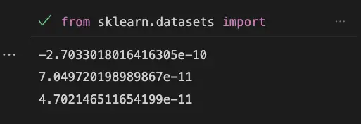
As we can see, the dot product between any two principal components is very close to zero, which indicates that the principal components are orthogonal.

Useful Python Libraries for Principal component analysis (PCA)

Here are some useful Python libraries and their methods that can be used for Principal Component Analysis:

• scikit-learn: PCA
• NumPy: cov, eig
• Pandas: DataFrame, corr
• Matplotlib: scatter

scikit-learn: is a popular Python library for machine learning, which provides an implementation of PCA through the PCA class.

NumPy: is a numerical computing library in Python. It provides functions to compute the covariance matrix and eigenvectors of a given dataset, which are required for PCA.

Pandas: is a data manipulation library in Python. It provides the DataFrame object, which can be used to store and manipulate tabular data. It also provides the corr method to compute the correlation matrix of a given dataset.

Matplotlib: is a plotting library in Python. It provides various types of plots, including scatter plots, which can be used to visualize the data in the new coordinate system after applying PCA.

These libraries and their methods can be used to implement Principal Component Analysis in Python. For more information and examples, you can visit their respective documentation.

Datasets useful for Principal component analysis (PCA)

1. Iris dataset

from sklearn.datasets import load_iris
iris = load_iris()
X = iris.data
y = iris.target

2. Breast Cancer Wisconsin (Diagnostic) dataset

from sklearn.datasets import load_breast_cancer
cancer = load_breast_cancer()
X = cancer.data
y = cancer.target

3. MNIST dataset

from sklearn.datasets import fetch_openml
mnist = fetch_openml('mnist_784', version=1)
X = mnist.data
y = mnist.target.astype(int)

4. The digits dataset

from sklearn.datasets import load_digits
digits = load_digits()
X = digits.data
y = digits.target

Important Concepts in Principal component analysis (PCA)

• Covariance matrix
• Eigenvectors and Eigenvalues
• Singular value decomposition (SVD)
• Dimensionality reduction
• Explained variance
• Scree plot
• Orthogonality
• Centering and scaling data
• Reconstruction error
• Noise filtering
• Applications of PCA

Before Learning Principal Component Analysis (PCA)?

You should also know about these concepts if you really want to understand PCA:

• Linear algebra, including matrix multiplication, eigenvectors, and eigenvalues
• Multivariate statistics, including covariance and correlation matrices
• Basic knowledge of probability and statistics, such as mean, variance, and standard deviation
• Understanding of data preprocessing techniques, such as data normalization and standardization
• Familiarity with Python and its scientific computing libraries, such as NumPy, Pandas, and Matplotlib
• Understanding of machine learning concepts, such as supervised and unsupervised learning, feature extraction, feature transformation, feature engineering and dimensionality reduction.

What’s Next?

• Factor Analysis
• Multidimensional Scaling
• Independent Component Analysis (ICA)
• Non-negative Matrix Factorization (NMF)
• Manifold Learning
• Clustering Algorithms (K-means, Hierarchical, etc.)
• Feature Selection and Feature Extraction techniques

Questions People Often Ask About PCA

Conclusion

PCA is a powerful technique for dimensionality reduction and data analysis. It is widely used in machine learning, computer vision, and data analysis. PCA finds the most important features of the data, called principal components, and expresses the data in terms of those components. Although PCA has some limitations, it is a valuable tool in many applications.

Sources

• scikit-learn documentation on PCA
• PCA on Wikipedia
• Towards Data Science article on PCA
• Machine Learning Mastery article on PCA
• Python Data Science Handbook chapter on PCA
• Analytics Vidhya tutorial on PCA
• Tutorialspoint tutorial on PCA
• Medium article on PCA
• StatQuest video on PCA
• Jcchouinard’s PCA tutorial