Feature reduction is a critical aspect of machine learning involved in transforming features. It is involved in selecting the most relevant features from a dataset to improve model performance and reduce overfitting. In this article, we will discuss the importance of feature reduction, the different methods used for feature reduction, and the benefits of using feature reduction in machine learning.

Importance of Feature Reduction

In machine learning, the goal is to build a model that can accurately predict outcomes based on input data. However, many datasets contain hundreds or thousands of features, and not all of these features may be relevant for predicting the target variable. In fact, including irrelevant features can lead to overfitting, where the model learns to fit noise in the data rather than the underlying patterns.

Feature reduction is an effective way to overcome this challenge by selecting the most relevant features from the dataset, reducing the dimensionality of the problem, and improving model performance. It can also help to reduce computational costs and improve interpretability, making it easier to understand how the model is making predictions.

Methods for Feature Reduction

There are several methods for feature reduction in machine learning, including:

• Filter Methods: These methods involve selecting features based on statistical measures like correlation or mutual information. The most commonly used filter methods include Pearson correlation coefficient and chi-squared test.
• Wrapper Methods: These methods involve selecting features based on how well they perform in a given model. The most commonly used wrapper methods include forward selection, backward elimination, and recursive feature elimination.
• Embedded Methods: These methods involve selecting features as part of the model training process. The most commonly used embedded methods include Lasso and Ridge regression.

Benefits of Feature Reduction

The benefits of using feature reduction in machine learning include:

• Improved model performance: By reducing the dimensionality of the problem, feature reduction can improve model performance and reduce overfitting.
• Reduced computational costs: By reducing the number of features, feature reduction can also reduce the computational costs associated with training the model.
• Improved interpretability: By reducing the number of features, feature reduction can improve the interpretability of the model, making it easier to understand how it is making predictions.

Important Concepts in Feature Reduction (with Python Examples)

• Dimensionality Reduction
• Principal Component Analysis (PCA)
• Singular Value Decomposition (SVD)
• t-distributed Stochastic Neighbor Embedding (t-SNE)
• Linear Discriminant Analysis (LDA)
• Non-negative Matrix Factorization (NMF)

Dimensionality Reduction

This example uses Scikit-learn and matplotlib to visualize dimensionality reduction on the digits dataset.

from sklearn.datasets import load_digits
from sklearn.decomposition import PCA
import matplotlib.pyplot as plt

digits = load_digits()
X = digits.data
y = digits.target

pca = PCA(n_components=2)
X_reduced = pca.fit_transform(X)

plt.scatter(X_reduced[:, 0], X_reduced[:, 1], c=y)
plt.colorbar()
plt.show()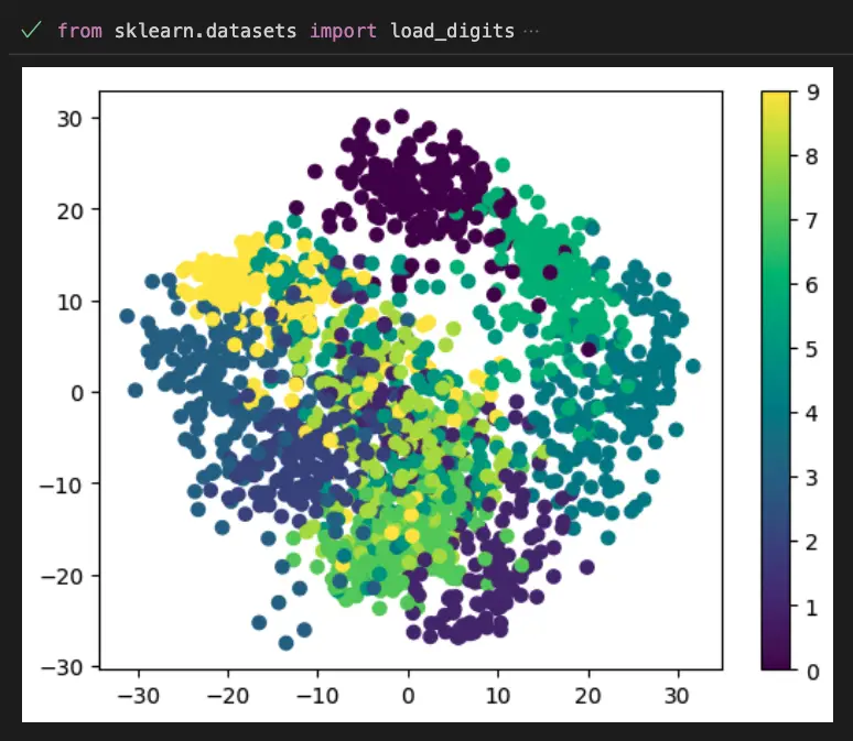

PCA Example in Python

This example uses Scikit-learn and matplotlib to visualize Principal Component Analysis on the iris dataset.

from sklearn.decomposition import PCA
from sklearn.datasets import load_iris
import matplotlib.pyplot as plt
# Load iris dataset
iris = load_iris()

# Create PCA object with two components
pca = PCA(n_components=2)

# Fit and transform data
iris_pca = pca.fit_transform(iris.data)

# Visualize data
import matplotlib.pyplot as plt
plt.scatter(iris_pca[:, 0], iris_pca[:, 1], c=iris.target)
plt.xlabel('PCA Component 1')
plt.ylabel('PCA Component 2')
plt.show()

This code first loads the iris dataset from scikit-learn, then performs Principal Component Analysis (PCA) for feature reduction. Finally, the reduced features are visualized using Matplotlib’s scatterplot function.

Singular Value Decomposition (SVD)

This example uses Scikit-learn, Seaborn and matplotlib to visualize Singular Value Decomposition on the digits dataset.

import seaborn as sns
from sklearn.datasets import load_digits
from sklearn.decomposition import TruncatedSVD
import matplotlib.pyplot as plt

digits = load_digits()
X = digits.data
y = digits.target

svd = TruncatedSVD(n_components=2, random_state=0)
X_svd = svd.fit_transform(X)

sns.scatterplot(x=X_svd[:,0], y=X_svd[:,1], hue=y, palette="deep")
plt.title("Singular Value Decomposition (SVD) using Seaborn")
plt.show()

t-distributed Stochastic Neighbor Embedding (t-SNE)

This example uses Scikit-learn and matplotlib to visualize t-SNE on the digits dataset.

import seaborn as sns
from sklearn.datasets import load_digits
from sklearn.manifold import TSNE
import matplotlib.pyplot as plt

digits = load_digits()
X = digits.data
y = digits.target

tsne = TSNE(n_components=2, random_state=0)
X_tsne = tsne.fit_transform(X)

sns.scatterplot(x=X_tsne[:,0], y=X_tsne[:,1], hue=y, palette="deep")
plt.title("t-distributed Stochastic Neighbor Embedding (t-SNE) using Seaborn")
plt.show()

Linear Discriminant Analysis (LDA)

This example uses Scikit-learn, Seaborn and matplotlib to visualize Linear Discriminant Analysis on the Iris dataset.

import seaborn as sns
from sklearn.datasets import load_iris
from sklearn.discriminant_analysis import LinearDiscriminantAnalysis
import matplotlib.pyplot as plt

iris = load_iris()
X = iris.data
y = iris.target

lda = LinearDiscriminantAnalysis(n_components=2)
X_lda = lda.fit_transform(X, y)

sns.scatterplot(x=X_lda[:,0], y=X_lda[:,1], hue=y, palette="deep")
plt.title("Linear Discriminant Analysis (LDA) using Seaborn")
plt.show()

Non-negative Matrix Factorization (NMF)

This example uses Scikit-learn and matplotlib to visualize Non-negative Matrix Factorization on the Digits dataset.

from sklearn.decomposition import NMF
from sklearn.datasets import load_digits
import matplotlib.pyplot as plt

digits = load_digits()
X = digits.data

nmf = NMF(n_components=2)
X_reduced = nmf.fit_transform(X)

plt.scatter(X_reduced[:, 0], X_reduced[:, 1], c=digits.target)
plt.colorbar()
plt.show()

Useful Python Libraries for Feature Reduction

• scikit-learn: PCA, LDA, NMF
• numpy: svd, eig
• pandas: drop, iloc, corrcoef

Datasets useful for Feature Reduction

UCI Wine Quality Dataset

# Load the dataset
from sklearn.datasets import load_wine
data = load_wine()
#Separate features and labels
X = data.data
y = data.target

UCI Breast Cancer Wisconsin (Diagnostic) Dataset

# Load the dataset
from sklearn.datasets import load_breast_cancer
data = load_breast_cancer()
#Separate features and labels
X = data.data
y = data.target

UCI Machine Learning Repository – Spambase Dataset

# Load the dataset
import pandas as pd
data = pd.read_csv('https://archive.ics.uci.edu/ml/machine-learning-databases/spambase/spambase.data', header=None)
#Separate features and labels
X = data.iloc[:, :-1]
y = data.iloc[:, -1]

Things You Should Know Before Diving into Feature Reduction

• Basic understanding of linear algebra and matrix operations
• Knowledge of statistical techniques such as covariance and correlation
• Familiarity with different types of machine learning algorithms and how they use features
• Understanding of the bias-variance tradeoff
• Familiarity with Python programming and relevant libraries such as NumPy, Pandas, and Scikit-Learn

What’s Next?

• Feature Engineering
• Feature extraction
• Feature selection
• Dimensionality reduction
• Clustering
• Anomaly detection
• Classification
• Regression
• Neural networks
• Deep learning models

Relevant entities

Entity	Properties
Dataset	Contains the data used to train the model
Features	The variables that represent the characteristics of the data
Dimensionality	The number of features in a dataset
Overfitting	When a model is too complex and fits the training data too closely, leading to poor generalization to new data
Principal Component Analysis (PCA)	A technique used for reducing the dimensionality of a dataset by finding the principal components that explain the most variance in the data
Linear Discriminant Analysis (LDA)	A technique used for feature reduction by projecting the data onto a lower-dimensional space that maximizes the separation between classes

Frequently Asked Questions

Conclusion

Feature reduction is an essential aspect of machine learning that can help to improve model performance, reduce overfitting, and improve interpretability.

There are several methods for feature reduction, including filter methods, wrapper methods, and embedded methods. By selecting the most relevant features from the dataset, feature reduction can help to improve the accuracy and efficiency of machine learning models.

Sources

Wikipedia page on Feature Selection and Feature Extraction: https://en.wikipedia.org/wiki/Feature_selection and https://en.wikipedia.org/wiki/Feature_extraction

Scikit-learn documentation on Feature Selection and Dimensionality Reduction: https://scikit-learn.org/stable/modules/feature_selection.html and https://scikit-learn.org/stable/modules/decomposition.html

Towards Data Science article on Feature Reduction: https://towardsdatascience.com/feature-reduction-techniques-87378c129e36

Analytics Vidhya article on Feature Selection and Feature Extraction: https://www.analyticsvidhya.com/blog/2020/10/feature-selection-techniques-in-machine-learning/

Machine Learning Mastery article on Dimensionality Reduction: https://machinelearningmastery.com/dimensionality-reduction-for-machine-learning/